Abstract
The Nobel Prize in Physics, Chemistry, and Physiology or Medicine is awarded once a year to scientists whose work a committee in Stockholm has judged to be sufficiently important. We ask a narrower question: among scientists good enough to plausibly win one, what predicts how long they wait? We assemble a pool of 1,043 candidates from the Wolf Prize, the Lasker Award, the Gairdner Award, and the Clarivate Citation Laureates and fit a Bayesian Weibull accelerated-failure-time model with two competing hazards, one for winning and one for dying first. By raw effect size, the two largest predictors of wait time are not citations, institutional prestige, or field: they are how quickly a discovery was first recognised by a precursor prize, and the scientist's first name. The first of these has an obvious explanation. The second does not. The least surprising finding in this paper is also the most robust: once name, mentorship, and recognition lag are accounted for, where you trained and how many papers you wrote add almost nothing. Hitherto, none of this will surprise a working scientist. We publish it anyway.
Introduction
Once a year, a committee of Swedish academics decides whose contributions to human knowledge are worth ten million kronor, a medal, and a black-tie dinner in a city that is dark by three in the afternoon in December. The Nobel Prize was created by Alfred Nobel, inventor of dynamite, who, upon reading his own premature obituary in a French newspaper that remembered him, unflatteringly, as "the merchant of death", reportedly concluded that a sufficiently large philanthropic action might improve his legacy. It has, on balance, worked. The Nobel Prize is now the closest thing science has to being knighted. The prizes are, generally, well regarded. They are not, however, without a certain historical texture.
Consider Enrico Fermi, awarded the 1938 Physics prize for producing new radioactive elements via neutron irradiation. This was an elegant result. It was also wrong: Fermi's team had been splitting uranium nuclei, so nuclear fission, and mistook the fragments for new transuranic elements. The committee announced the prize in November 1938. Otto Hahn, Fritz Strassmann, and Lise Meitner correctly worked out what had actually happened the following month. The prize was not revised. Fermi, to his credit, went on to help build the world's first nuclear reactor, which suggests he took the correction well.
Next, consider António Egas Moniz, awarded the 1949 Physiology or Medicine prize for the prefrontal leucotomy, the lobotomy, a procedure that severed connections in the prefrontal cortex, frequently without consent by the patient, disproportionately performed on women, and reliably producing permanent neurological damage. The committee called it one of the most important psychiatric discoveries ever made. The procedure is now banned across most of the world.
And finally, the double helix. In 1962, James Watson, Francis Crick, and Maurice Wilkins received the prize for the structure of DNA. The work drew heavily on X-ray crystallography data produced by Rosalind Franklin, without her being involved in the decision to use it. Franklin had died four years earlier, which, under the rule against posthumous prizes, would have excluded her from consideration regardless of how the credit had been assigned.
There are, in addition, scientists considered overdue who have not received the prize; scientists who received it before their work's importance was understood; scientists who made the key contribution but shared it with collaborators who were honoured and collaborators who were not; and scientists who made the key contribution but were at the wrong institution, in the wrong field, with the wrong advisor, or, and this is the subject of this post, with the wrong first name.
The question I want to ask is narrower than "who deserves a Nobel Prize," which we are not equipped to answer and which the Swedish Academy has spent answering imperfectly for over a century. We ask instead: among scientists good enough to plausibly win one, what predicts how long they wait? That is a different question from what predicts winning at all, and it calls for a different statistical tool: survival analysis, run the Bayesian way.
Data & Methods
Who Gets to Wait. To study who wins a Nobel Prize, you first need a list of people who might plausibly win one. "Every living scientist" is correct, but useless. I, as a PhD student for example, would, put humbly, of course be perfectly qualified for receiving a Nobel, yet the meager 2 citations on my last paper at the time of writing are not enough for any Swedes to get wind of me. Thus, we instead use a pool of 1,043 candidates assembled from the winners of the Wolf Prize, the Lasker Award, the Gairdner International Award, and Clarivate's Citation Laureates list. Together they function as the Nobel committee's waiting room: pre-filtered for quality, which lets us ask what else, beyond quality, predicts the timing.
Of the 1,043 candidates, 655 went on to win a Nobel Prize. Ninety-five died before they could. The remaining 293 are still in the waiting room: alive, prize-free, and, we can assume, checking their email or mobile every October.
Figure 1 shows what "waiting" looks like in practice: the bigger the bubble, the longer someone sat in the queue. Laureates typically make their defining discovery in their late thirties to early forties, then wait a mean of 19.5 years before the call comes, collecting the prize in their late fifties. The shortest wait on record belongs to Chen Ning Yang and Tsung-Dao Lee, who proposed parity violation in 1956 and were awarded the prize in 1957. Recognised, more or less, before most of the field had finished reading the paper. The longest wait on record is harder to assign, because some candidates are still accumulating it. This can be seen in the figure above. In recent years there has been an increase in the age and subsequently waiting time of laureates, some being over 90 years.
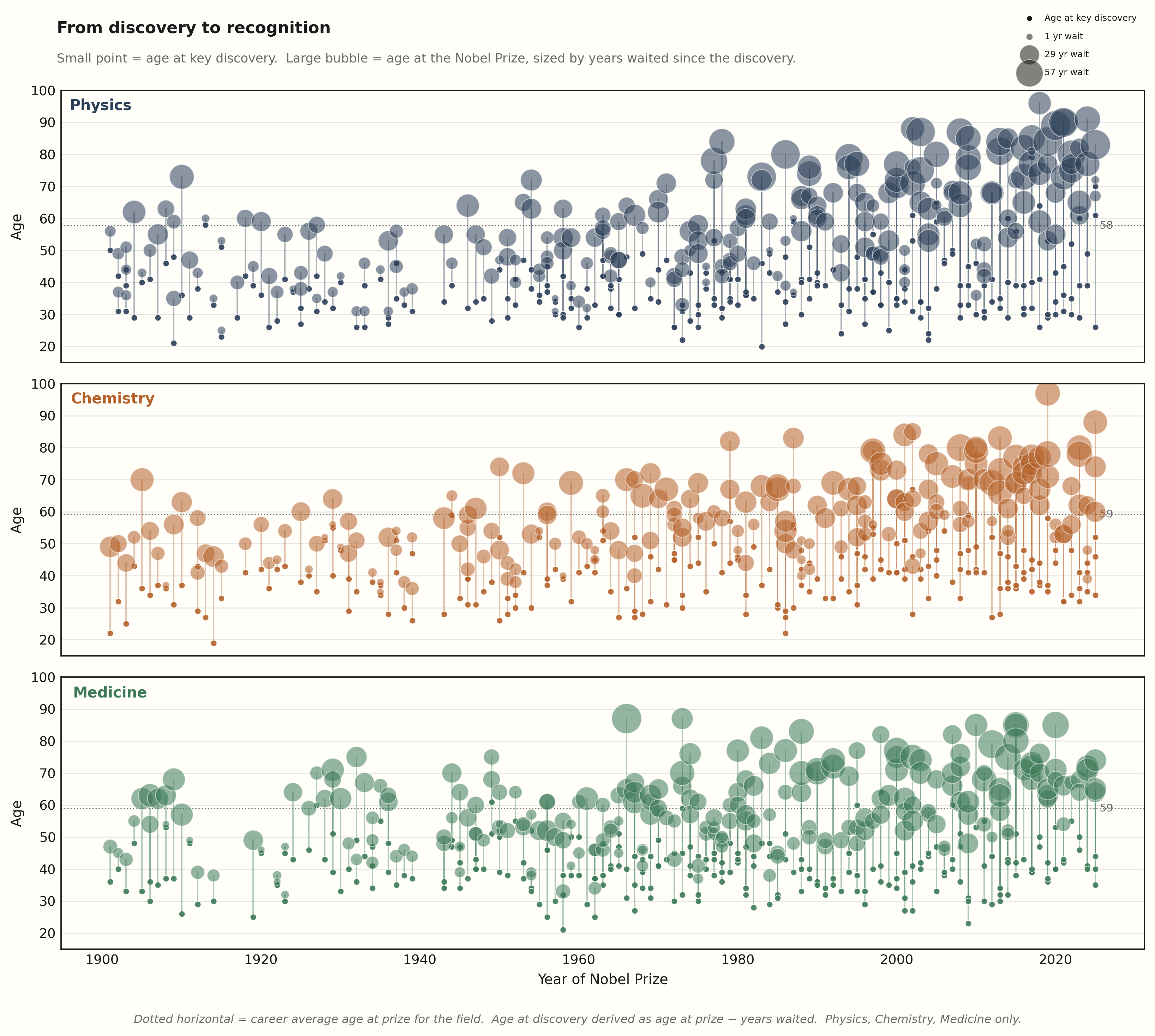
Figure 1. For each laureate: a small point marks age at the key discovery; a larger bubble marks age at the Nobel Prize, sized by years waited between the two. The dotted line marks each field's career-average age at the prize.
It's tempting to imagine that a scientist accumulates something like pressure toward eventual recognition and that enough pressure eventually produces a Nobel Prize, provided the candidate survives long enough to collect it. That second clause turns out to matter a great deal, and it's the entire subject of the next section.
Any working scientist without a permanent position will recognise that it is entirely to appropriate to transfer this framework to their current professional situation as well.
Two Ways to Leave the Room. The standard tool for modelling "how long until an event happens" is survival analysis, so named because it was developed to model time until death and never quite dropped the vocabulary. The relevant unit is the hazard: the instantaneous risk that the event happens at time
In our case, nobody (mostly) is dying of anything. We're modelling time until a phone call from Stockholm, not time until death. As it turns out, though, we need to model both, for reasons that are about to become clear.
We can define
- Nobel (655 candidates): they won.
runs from discovery to prize year. - Death (95 candidates): they died without winning.
runs from discovery to death year. - Censored (293 candidates): we don't know how their story ends. They are alive, have not won, and
runs from discovery to the present. This is right-censoring. It is not missing data, but more like incomplete data: we know they haven't won yet, and that's the entire content of the observation.
It's tempting to combine the dead with the censored. Both groups, after all, have the "not won" flag in common. However, as the Nobel Prize cannot be awarded posthumously, a candidate who died in 1985 is not "still waiting" in 2026; their probability of a future Nobel is exactly zero. Treat death as censoring, and the model concludes that quite some very old, very long-waiting candidates have an excellent shot any day now, because it has lost the ability to distinguish "old and still in the running" from "deceased."
The fix is a cause-specific competing-risks model: two separate hazards sharing the same clock, one for "wins the Nobel," one for "being dead." Each candidate contributes to the likelihood according to how they actually exited. A win counts as an event for the Nobel hazard and a survival for the death hazard, and vice versa for a death, while a still-waiting candidate has survived both. The death hazard itself is kept minimal on purpose, driven mostly by age at discovery; its only job is to correctly remove the deceased from contention.
Bayesically Estimation. To model each hazard, we use a Weibull accelerated failure time (AFT) model. The Weibull part is a flexible family of curves describing how risk changes over the course of waiting. It can represent a hazard that starts low and accelerates, or starts high and tails off, depending on what the data want. The "accelerated failure time" part is the useful bit for interpretation: instead of asking how a predictor changes the instantaneous risk at every moment (which is what a Cox model would do), an AFT model asks how a predictor stretches or compresses the entire timeline. Picture time as a treadmill: an AFT model doesn't change the shape of your run, it changes how fast the belt moves underneath you.
That framing produces a simple output: a time ratio,
We fit this the Bayesian was, which bayesically (this never gets old) changes what kind of answer you get back. A frequentist version of this model would hand you a single best-guess coefficient and a confidence interval whose correct interpretation nobody at the dinner table actually wants explained to them. A Bayesian model instead returns a full posterior distribution meaning the entire range of coefficient values consistent with the data, weighted by how plausible each one is. From that we can report the 89% highest density interval (HDI): the narrowest band containing 89% of that plausible range. A result counts as a real effect in this post when its HDI clears 1.0 entirely on one side. A result is "inconclusive" when the HDI touches 1.0. This means, the data cannot tell us whether the effect speeds things up, slows them down, or does nothing at all.
The 89%, instead of the more familiar 95%, is a small piece of statistical theatre: a deliberately odd number, chosen specifically so nobody mistakes it for a magic threshold. Bayesians do this to one another on purpose.
For the methodologically anxious: this model converged cleanly. Zero divergent transitions, a maximum r-hat of 1.002 across every parameter, a minimum effective sample size above four thousand. Whatever you make of the conclusions below, the sampler was not confused while producing them.
Results: How to shorten your wait.
Your Name influences the Wait. Figure 2 shows the distribution of the posterior effect of each predictor. Let's go through them step by step. Two predictors dominate the model, in opposite directions, for very different reasons.
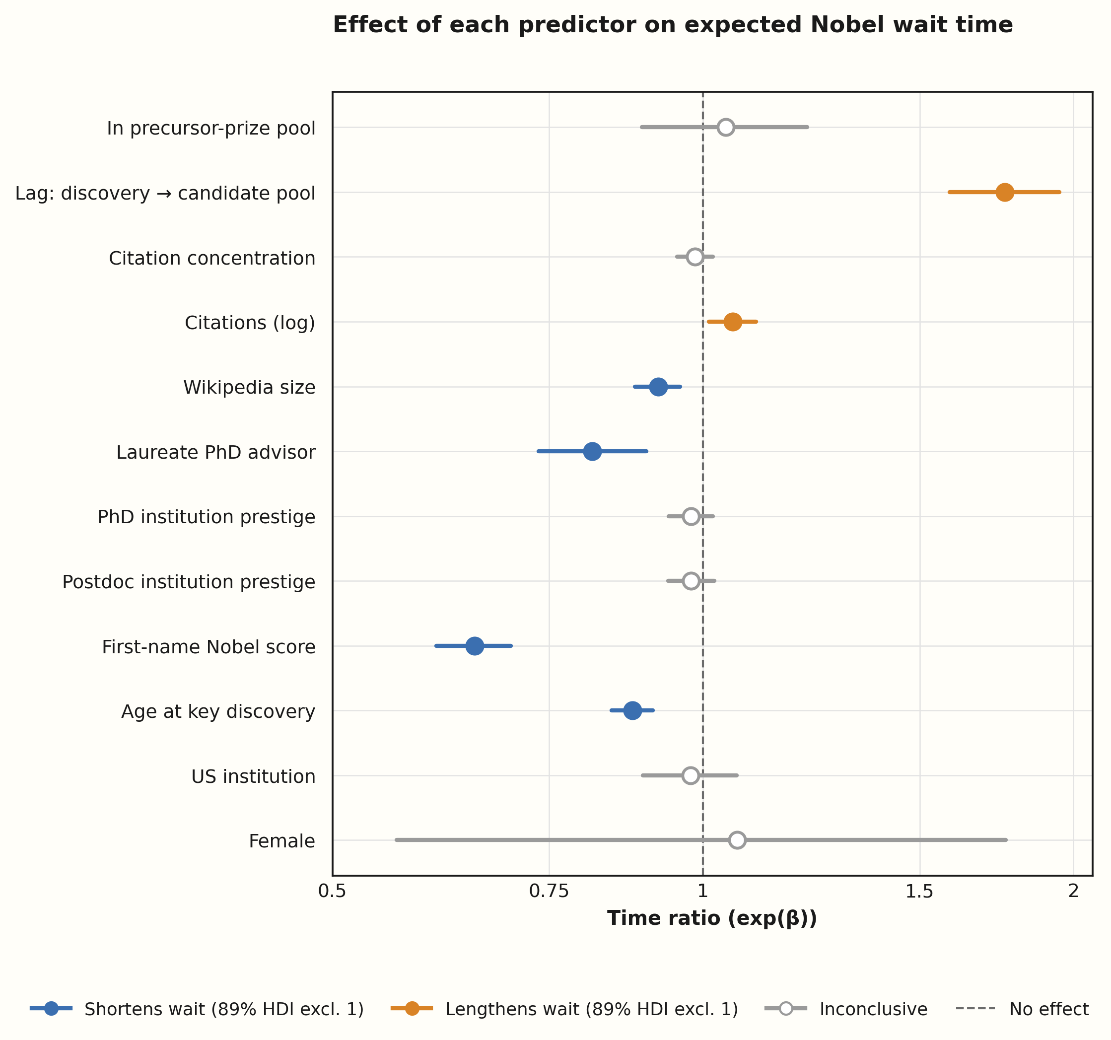
Figure 2. Posterior time ratios for every predictor in the model. Points are posterior means; horizontal lines are 89% HDIs. Filled markers indicate the HDI excludes 1 — blue shortens the wait, orange lengthens it; open grey circles are inconclusive.
Lag from discovery to candidate pool (TR = 1.76) is, by raw effect size, the single largest coefficient anywhere in the model. Every additional standard deviation of delay between a scientist's key discovery and their first precursor-prize recognition (a Wolf, Lasker, Gairdner, or Clarivate nod) multiplies the expected Nobel wait by 1.76. This means, if the first set of judges took decades to notice you, the second set probably will too. Sorry.
First-name Nobel score (TR = 0.65) is the second-largest effect, and the more interesting one, because it has no equivalent one-sentence explanation. A scientist whose first name sits at the favourable end of the historical laureate distribution can expect to wait roughly a third less time than an otherwise identical scientist whose name does not. There is no honest causal story here, which is the entire point, and the subject of its own section below.
Having a Nobel laureate as a PhD advisor (TR = 0.81) and age at key discovery (TR = 0.88) come next. Both clearly significant, both smaller than the two effects above. Training under someone who already got the call shortens the wait; so does making your discovery younger, plausibly because earlier discoveries have more time to accumulate replication and consensus before a committee has to act.
Wikipedia article size (TR = 0.92) also clears the bar, but only just. A larger cultural footprint helps, at least a bit. But please, as someone who is working on some articles, please, I beg you, please do not go and expand your own article at will.
Lastly, are citations, which behave not as how you'd guess. Total citation count, log-scaled, comes in at TR = 1.06. This is small, but reliably on the wrong side of 1: more citations, slightly longer wait. The best guess would be that broad, diffuse career impact is harder for a committee to pin on one defining contribution than a single, legible breakthrough is. We built a separate variable specifically to test that theory directly: Citation concentration, the share of a candidate's citations coming from their single most-cited paper. And it does not clear the bar (TR = 0.99, HDI comfortably crossing 1, too bad).
Everything else is inconclusive: PhD and postdoc institution prestige, US institutional affiliation, simply having entered the precursor-prize system at all (as distinct from how long it took to get there, which very much matters), and the gender coefficient.
Once name, mentorship, and recognition lag are accounted for, where you trained and how many papers you published add essentially nothing. This will not surprise anyone who has sat through a grant panel.
The John Problem. Let's come back to the more questionable finding: the first name. Or as I call it: the John problem. As seen in Figure 3, John leads with 25 laureates, and the curve is still climbing: he'd reached 13 by the year 2000 and doubled that in the twenty-five years since. Robert, George, Paul, William, Richard, James, and David constitute the top eight, and between them they account for a genuinely large fraction of twentieth- and twenty-first-century science.
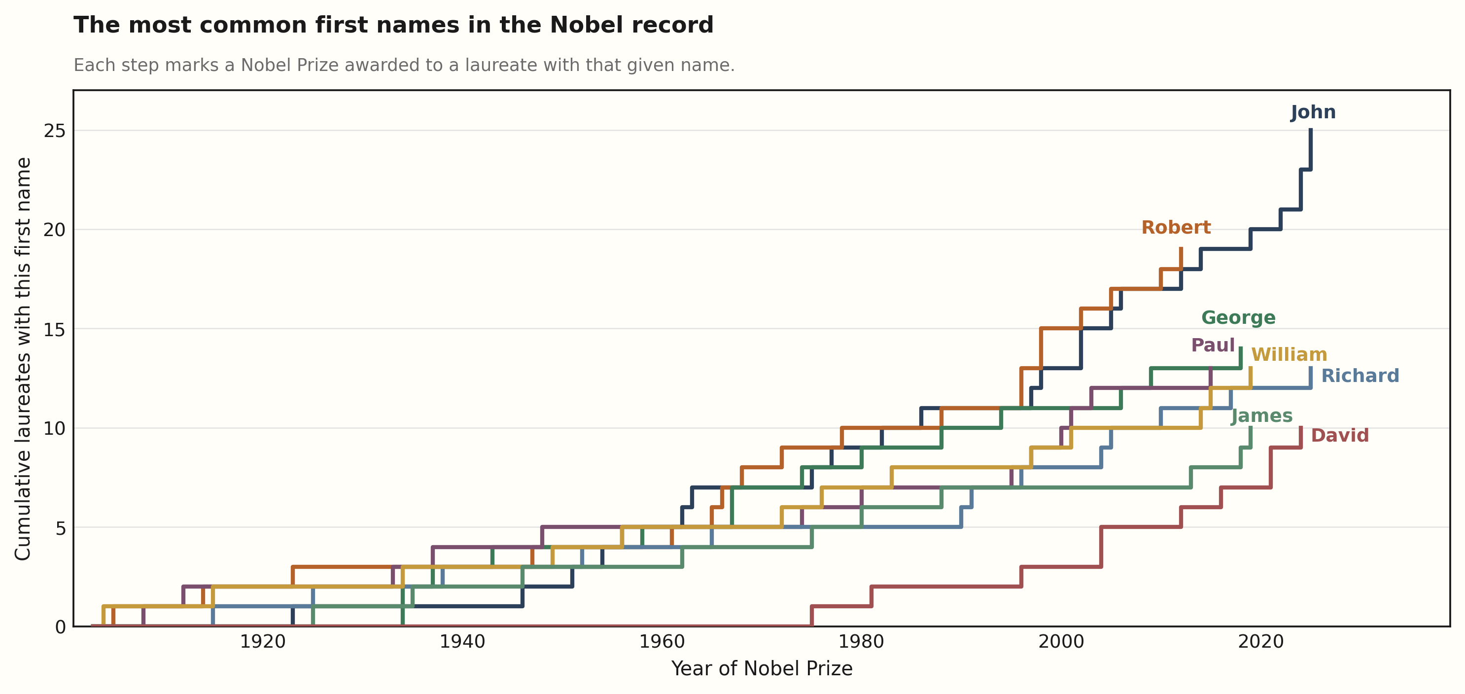
Figure 3. Cumulative Nobel count for the eight most common first names among laureates. Each step is one prize.
To be clear about what this actually means: Of course, just because your name is John you are not automatically higher on the minds of the committee. What we instead measured was the extent to which twentieth-century Nobel mentorship has been an Anglo-American family business and a first name is simply the cheapest available marker for that. A model cannot separate "John" from "the kind of person, trained in the kind of network, in the kind of country and decade, who was statistically likely to be named John". Put bluntly: "John" is along for the ride on a Nobel Prize that, for most of the twentieth century, was substantially a US and UK production with occasional international guest stars.
Geography. However, this was not always the case. Figure 4 shows the share of Nobel Prizes received by scientists born in a specific country. Germany dominated the early twentieth century, see the wide grey band sitting above a barely visible sliver of dark navy in the 1910s. That sliver, the United States, now accounts for roughly half of all laureates, and the two lines cross somewhere around the run-up to the Second World War. This is a coincidence of timing that requires no further commentary from us.
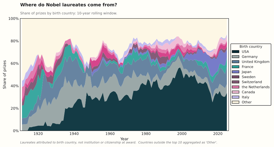
Figure 4. Share of prizes by laureate birth country, ten-year rolling window. Countries outside the top ten are pooled as Other.
And yet, once name, mentorship, and recognition lag are in the model, institution prestige and national affiliation drop out almost entirely as predictors of wait time. They may well predict whether someone enters the candidate pool in the first place. They don't predict how long the wait is once they're in it. Geography shapes the field; on this evidence, it doesn't shape the stopwatch.
Who's Next. After having put in the effort to model what influences wait time, it would be a pity, not to use this knowledge to make a prediction on who, according to the model, has the highest chance of winning in the coming 10 years. At the time of writing, you can bet on almost anything, but please, don't use this information to place your bet. Keep in mind the name of this humble journal.
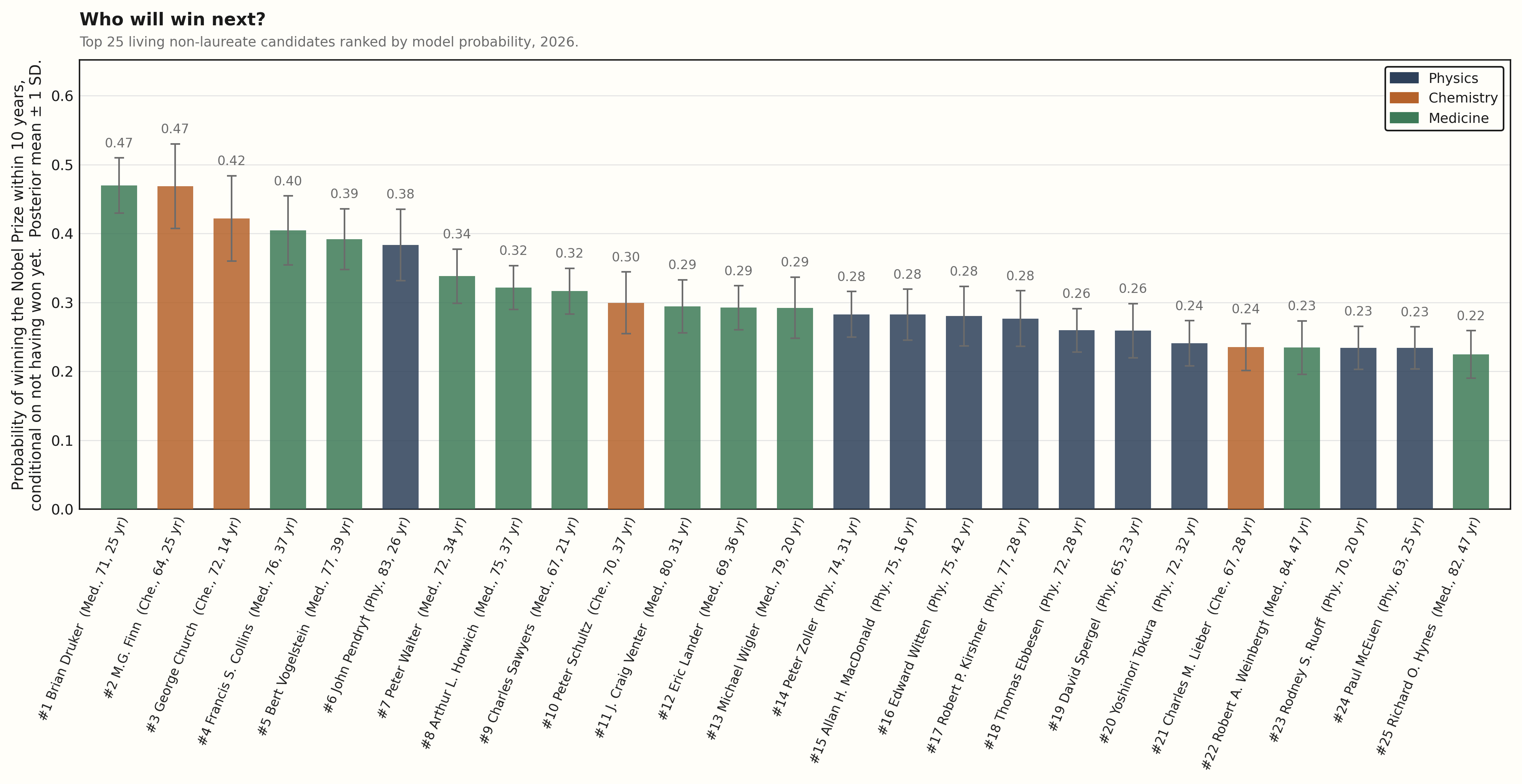
Figure 5. Top 25 living non-laureate candidates, ranked by posterior probability of winning within 10 years. Error bars are ±1 posterior SD.
Essentially, This figure justifies the entire detour into competing-risks modelling. If not for the competing risks, the model put a 101-year-old Medicine candidate in first place, with a modelled win probability of 0.80, purely on the strength of having waited longer than almost anyone else in the dataset. The model had no way to penalise that wait for the fact that the candidate's remaining time to actually receive a phone call was running out faster than their accumulated case for receiving one was growing. That's what happens when "still waiting" and "running out of road" share a bucket: the ranking turns into a list sorted by age, not by merit.
With the death hazard properly separated out, the ranking changes considerably. Brian Druker and M.G. Finn now share the top spot at 0.47, followed by George Church (0.42), Francis Collins (0.40), and Bert Vogelstein (0.39), each combining a favourable structural profile (an early discovery, a laureate-lineage advisor, rapid community recognition) with a wait that hasn't yet started running against their biological clock. Conspicuously absent from the top of the corrected list: anyone whose primary qualification was simply having waited an extremely long time.
Discussion and Conclusion
A few honest limitations first, in the interest of not overselling a Weibull model fit to 1,043 people: The candidate pool is itself a selection. The Wolf, Lasker, Gairdner, and Clarivate committees do not pick candidates at random, and if the same structural advantages (name, mentorship, visibility) that speed up the second gate also helped a candidate through the first one, our predictors describe what gets you through the system, not necessarily what makes the science good. We have not corrected for this, because doing so honestly would require a model of committee behaviour we do not have and probably do not want.
The first-name effect, specifically, is simply a proxy for Anglo-American dominance in Nobel mentorship networks, not a literal name effect, and you should not consider changing your first name to get a Nobel Prize.
However, none of this will get Rosalind Franklin her Nobel Prize, decades too late and several years too dead to have qualified under the rules that excluded her anyway. It will, however, tell you roughly who to keep an eye on this October.
Preferably someone named John.
Acknowledgements
This post was heavily inspired by BobbyBroccoli, whose excellent three-part documentary explores the story of a man who came remarkably close to faking his way to a Nobel Prize. Beyond being a fascinating account of scientific fraud, it also does a wonderful job of sketching the profile of a typical Nobel laureate and the institutions that surround them.
You can watch it here
It is both informative and genuinely hilarious.